CAL-P: Application note
1. Introduction
The validity of the results of environmental electromagnetic field measurements (whether the electric or magnetic component, or the power density) depends not only on the periodic calibration (annual or biennial) of the sensors, but also on maintaining their performance between one calibration and the next.
As indicated in the ISO/IEC 17025 guideline (Chapters 6 and 7) and in ILAC G24 (“Guidelines for the determination of calibration intervals of measuring instruments”), it is essential to implement intermediate checks to confirm the calibration status of the instrumentation.
This is particularly critical for broadband probes and selective antennas, which are subject to mechanical stress, component ageing and environmental variations during outdoor measurement activities, in addition to potential damage during measurement campaigns.
Intermediate checks are very often neglected and, when they are performed, they are mostly managed with limited awareness of the reliability of the method employed.
This document is intended to assess the reliability of the CAL-P verification system so as to make its repeatability and dependability evident, primarily by stating its measurement uncertainty.
2. The CAL-P System
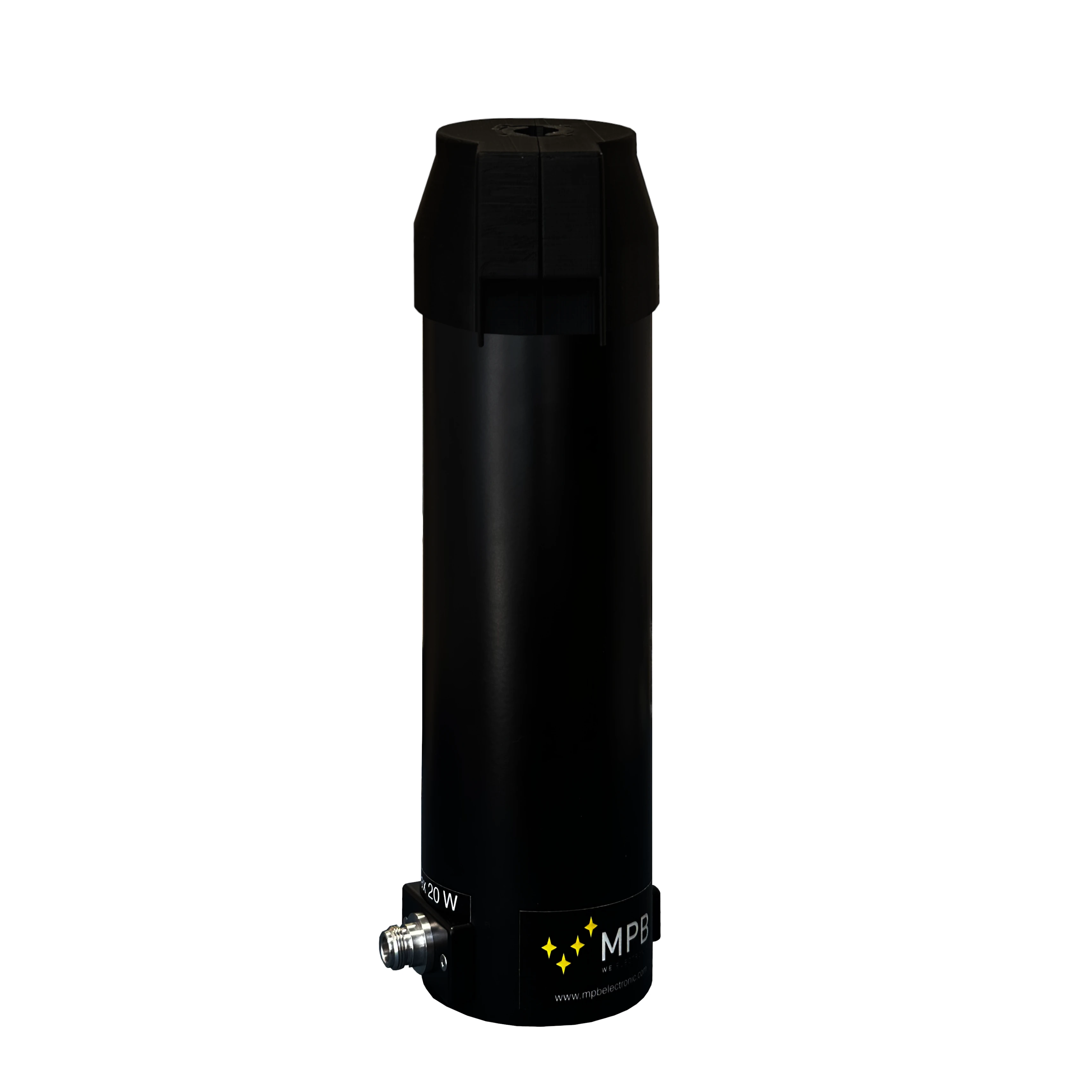
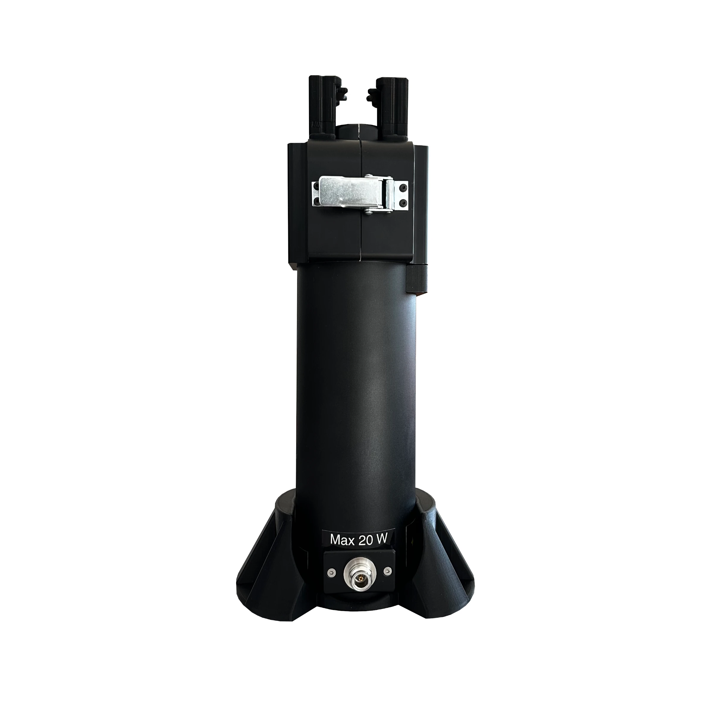
As detailed more fully in the CAL-P system datasheet, the above checks can be carried out autonomously and repeatably thanks to a “shielded RF chamber” (Jig) and an integrated signal generator.
Two distinct procedures can be adopted, which in this context we shall call V-dedicate and V-statistic.
V-dedicate: after the probe has undergone its scheduled calibration according to the calibration plans, or immediately after purchase, it is inserted into the Jig chamber and a measurement is performed which is adopted as the reference. For each frequency selected at this stage, the field value is read and a maximum permissible “error” value is associated with it. The acceptance limit set for each frequency must be commensurate with the verification uncertainty quantified in this document (see Sec. 4).
Subsequently, according to the time schedule of intermediate checks, or whenever doubts arise about the actual operation of the probe/antenna, the probe is re-measured by the CAL-P system at the same frequencies and the current curve is compared with the reference one: if the deviation, frequency by frequency, falls within the set limit, the system returns PASS, otherwise FAIL.
The comparison is performed for all the frequencies defined during acquisition of the reference curve.
V-statistic: exploiting a predefined statistical analysis as a function of the specific probe model under test, the re-reading phase that confirms (or not) the intermediate check is in practice compared with the population band of the model.
Adopting this methodology yields, besides a practical advantage — avoiding a reference curve for every probe to be verified — also the confirmation of the probe’s compatibility with the population of its model. This is significant because it provides a common verification baseline.
For example, for a control body that performs environmental measurements and owns several probes of the same model, this method allows an effective and non-empirical check over the entire probe fleet.
At present, the statistical characterization is available for the EP745 probe (a sample of 9 units), and in particular the frequencies of 500 MHz, 1750 MHz and 3 GHz have been adopted.
The three frequencies were selected by MPB according to a “trade-off” criterion among: lower variability across the serial numbers of the model, stability in repeatability, and coverage of the frequency bands most commonly present in the environment.
In this case too, a PASS/FAIL criterion is adopted, which in practice takes into account the width of the acceptance band (see Sec. 4).
In both modes, the repeatability of the positioning — depending on the specific probe/antenna under test — is ensured by specific geometric reference points of the particular Jig supplied.
Reference is made to the system datasheet for a fuller understanding of its operation. The purpose here is instead to analyse and quantify the measurement uncertainty in the two verification modes.
3. Uncertainty evaluation according to JCGM 100:2008 (GUM)
The aim here is to analyse the various contributions making up the uncertainty in the use of the CAL-P system, proceeding to the analysis of the combined uncertainty according to the GUM approach (JCGM 100:2008).
Consideration is given to the uncertainty in the repeatability both of the positioning of the same probe in the Jig system and of the measurement of the electromagnetic field value performed on a sample of probes of the same model, in addition to the uncertainty in the time stability of the signal generator that is part of the CAL-P system and in its reproducibility.
3.1 Type A uncertainty
This contribution derives from the statistical variability observed during repeated tests and is evaluated, for each preset frequency fᵢ, from the series of N readings acquired under the same conditions.
The same rationale applies both to the repeated measurements of N probes of the same model (V-Statistic) and to the positioning repeatability of the single probe.
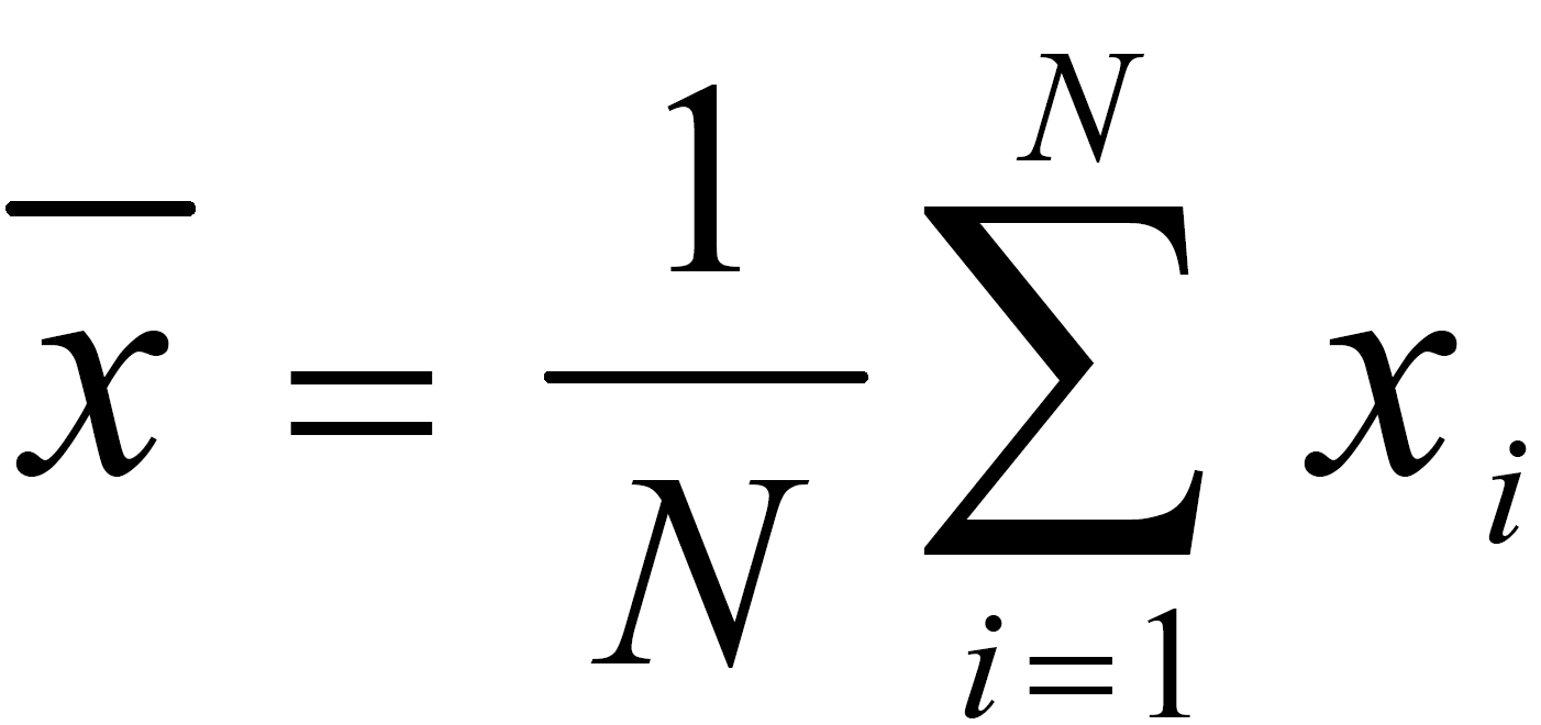
The mean value of the N measurements is computed:
The experimental standard deviation of the mean (1σ):
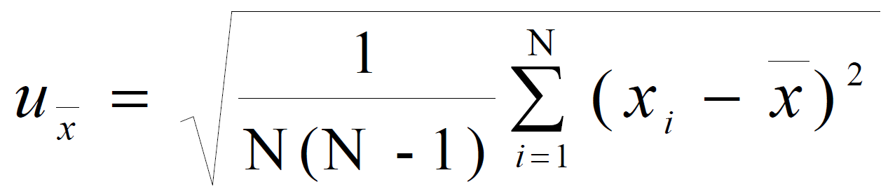
ux̄ is the uncertainty with which the mean value is known, a factor √N smaller than the dispersion of the single reading.
For the subsequent conversion to dB (cf. Appendix A) it is convenient to express the contribution in relative form:
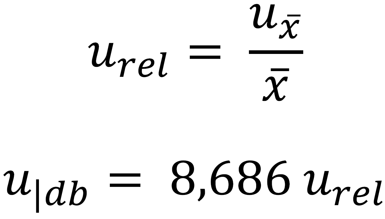
This contribution has been evaluated both for the positioning repeatability of the probe in the Jig and for the measurements performed on the sample of probes of the same model.
3.1.1 Positioning repeatability
Thanks to the guided fastening of the probe in the Jig and to the experimental confirmations (20 insertion/extraction cycles), an uncertainty u_pos (1σ)
u_pos = 0.08 dB (about 1% — see Appendix A).
3.1.2 Repeated measurements of N probes of the same model
This evaluation is indicative for a family of Narda probes, in particular the EP745 model. It may undergo numerical changes depending on the “stability” of the population of the model to be statistically characterized. From the experimental confirmations performed on 9 EP745 probes it was possible to obtain, as a maximum, at the three selected frequencies (0.16 dB at 500 MHz, 0.27 dB at 1750 MHz, 0.23 dB at 3 GHz), a Type A uncertainty equal to the experimental standard deviation of the mean.
u_mod_max = 0.27 dB
3.1.3 Uncertainty due to the reproducibility of the RF generator
A contribution due to the reproducibility in the manufacture of the RF generator can be considered by adopting a Type A uncertainty contribution computed on 4 measurements. The contribution u_gen_reproducibility.
u_gen_reproducibility = 0.1 dB
These statistics will be extended by widening the measurements to several production lots, whose statistical analyses will allow a better estimate.
It should be noted that in this case, the number of measurements being relatively low, a Bayesian approach was preferred (cf. Appendix B).
3.2 Type B uncertainty (Generator Stability)
The contribution due to the time stability of the RF signal generator was evaluated from the technical specifications of the electronics employed and, conservatively, a rectangular probability distribution of half-width a=0.15 dB was adopted, obtaining an uncertainty contribution

3.3 Combined uncertainty
The combined standard uncertainty is obtained by combining the Type A and Type B contributions in quadrature:
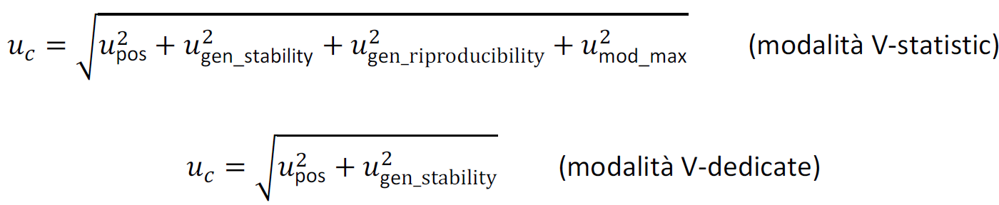
In the V-dedicate mode, the check is a differential comparison against the reference acquired in the same Jig and with the same generator; hence only the generator stability and the positioning repeatability remain in the budget.
| Contribution | V-dedicate | V-statistic | ν |
|---|---|---|---|
| Positioning repeatability (Type A) | 0.08 dB | 0.08 dB | 19 |
| RF generator stability (Type B) | 0.087 dB | 0.087 dB | ∞ |
| RF generator reproducibility (Type A) | — | 0.17 dB (Bayes.) | ∞ (Bayes) |
| Same-model probe variability (Type A) | — | 0.27 dB | 8 |
| u_c | 0.118 dB | 0.34 dB | |
| U at 95% | ≈ 0.24 dB (k = 2) | ≈ 0.7 dB (k = 2) | (*) |
In the V-statistic mode the dominant Type A contribution is the experimental standard deviation of the mean of the reference curve (N = 9, ν = 8). The reproducibility contribution of the RF generator with Jig is treated with the Bayesian approach (cf. Appendix B) and is multiplied by the factor √[(N−1)/(N−3)] = √3, obtaining 0.1 × √3 ≈ 0.17 dB. With this factor applied, all the contributions are combined in quadrature and k = 2 is adopted directly, without resorting to the computation of the effective degrees of freedom (Welch–Satterthwaite).
In the V-dedicate mode, the comparison being differential, the generator reproducibility and the same-model variability need not be taken into account, and the dominant contributions have high ν, so that k = 2 is directly applicable.
Note (*) The reproducibility component has been inflated according to the Bayesian approach (× √3), making it equivalent to an estimate with ν → ∞. The resulting effective degrees of freedom for the V-statistic mode (νeff ≈ 20, computed with the Welch–Satterthwaite equation) yield a factor t0.95 ≈ 2.09, entirely equivalent to the direct adoption of k = 2 for the final rounding to 0.7dB.
4. Acceptance criteria and decision rules
The deviation limit set during acquisition of the reference (V-dedicate mode) or the statistical acceptance band (V-statistic mode) are meaningful only if commensurate with the verification uncertainty (ILAC-G8, ISO 14253-1).
The practical recommendation is that the limit L be at least equal to 2–3 times the expanded uncertainty U of the verification: with the values assumed for the V-dedicate mode (U ≈ 0.24 dB), limits of the order of 0.5–0.7 dB ensure a contained decision risk under a simple acceptance regime. Likewise, for the V-statistic mode (U ≈ 0.7 dB) a factor of 2.5 leads to a limit of the order of 1.75 dB.
Alternatively, an explicit guard band can be adopted (PASS if Δ ≤ L − U).
5. Conclusions
The V-dedicate method proves metrologically superior: the differential nature of the comparison with the reference curve cancels systematic effects and the expanded uncertainty is limited to about 0.24 dB. It does, however, require the acquisition of the reference curve immediately after each calibration.
The V-statistic method is operationally more efficient: it does not require the acquisition of a dedicated reference curve for each probe, but compares the reading with the population band of the model, allowing a systematic and non-empirical control of the entire probe fleet. The expanded uncertainty is however larger (about 0.7 dB), since the budget also includes the variability among units of the same model and the reproducibility of the generator. It should also be borne in mind that it confirms the compatibility of the probe with the population of its model.
Appendix A — Propagation of “errors” from % to dB
A.1 Foreword
If an uncertainty U (at 2σ, for example) is expressed in %, in order to move to logarithms (e.g. dB) one cannot — obviously — apply the conversion formula as if it were a simple value. The uncertainty value indeed carries an associated probability distribution with a coverage factor: that is, it is a probabilistic value. For this reason the law of propagation of uncertainties (GUM, Chap. 5) must be applied to the % → dB transformation.
A.2 Model and sensitivity coefficient
The model of the transformation, considering the percentage value already normalized to 1, can be written as:

The partial derivatives must be applied to the model — in this case the simple derivative, since there is a single random variable contributing to the determination of the dB value. The sensitivity coefficient c₁ is therefore:
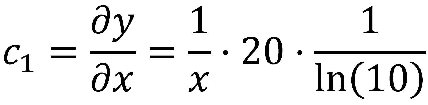
Useful reminders: for the change of base of logarithms, logₘ(a) = ln(a)/ln(b), i.e. log₁₀(x) = ln(x)/ln(10); the derivative of the natural logarithm is 1/x.
A.3 Combined uncertainty
Applying the law of propagation, the combined uncertainty is:

But since u(x)/x is the relative uncertainty — which in our cases is expressed in % and is relative to the value — we can conclude:

A.4 Example
Assuming a voltage measurement of 3 V with a relative uncertainty of 10% (normal distribution, 2σ), this is equivalent to having an uncertainty of:
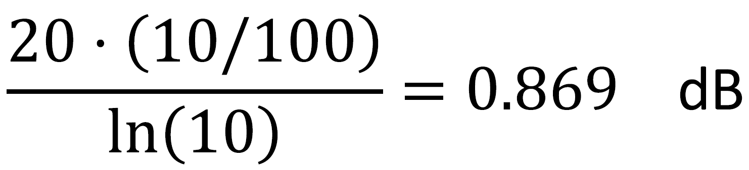
A.5 Two distinct worlds: measured values and uncertainties
It is important not to confuse two conceptually different planes.
Measured values and deviations — always mean or estimated values, i.e. deterministic numbers — are converted with the direct transformation formulas:
For field quantities (V/m, A/m):

For power quantities (W/m²):

The associated uncertainties are instead probabilistic values — they carry with them a probability distribution and a coverage factor — and are converted exclusively with the propagation law derived in §A.3:
For field quantities (V/m, A/m):
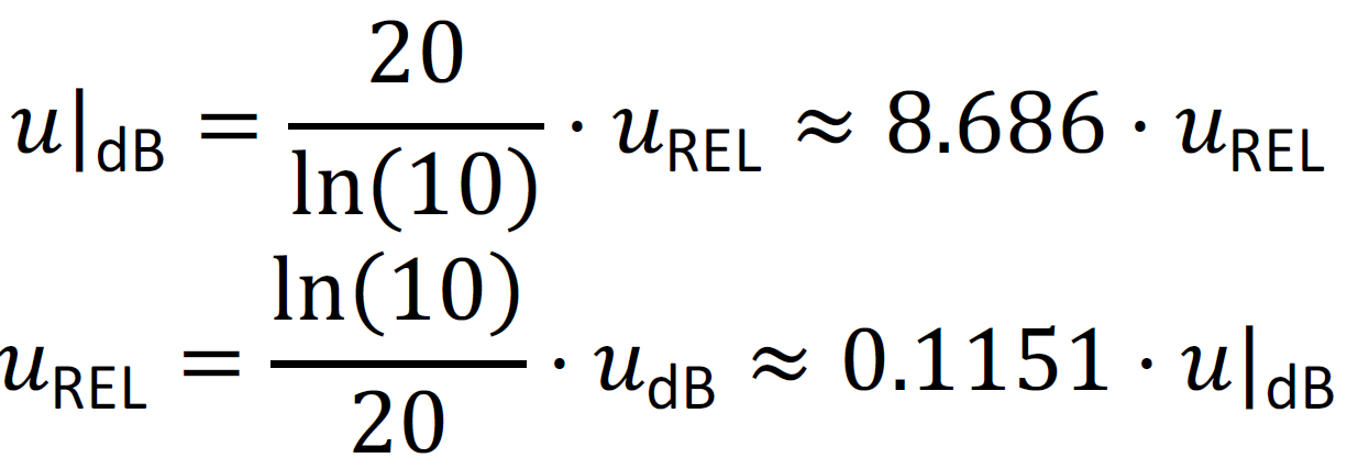
For power quantities (W/m²):
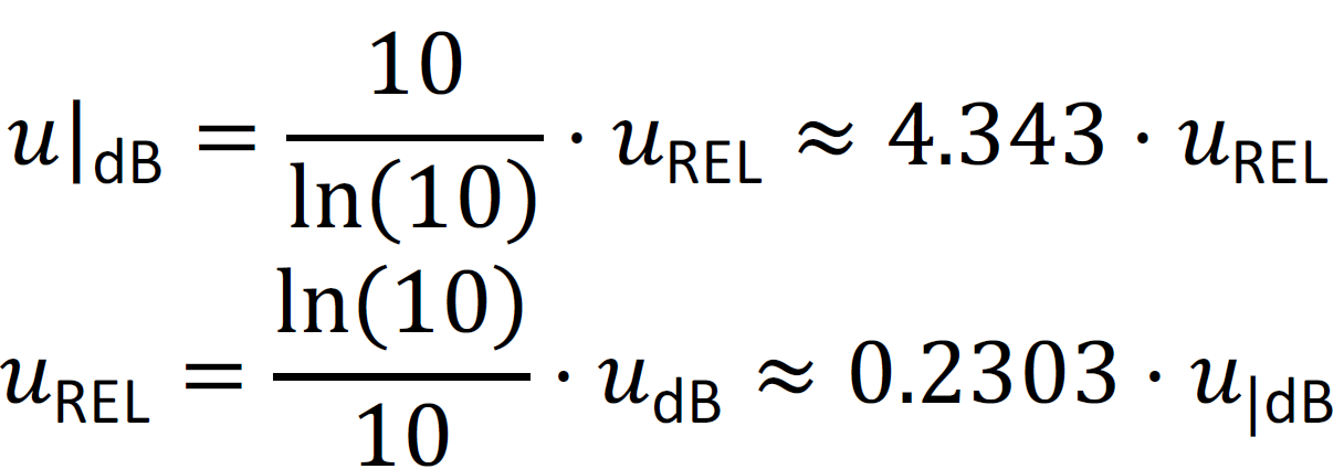
Mistakenly applying the value-conversion formulas to the uncertainties produces numerically small deviations when the uncertainties are small, and increasingly relevant ones as the uncertainty grows; but the point is not the size of the error. One thing is the value of the measurements or of the deviations, the uncertainty associated with them is another: they are two different worlds, and each has its own conversion formula.
Appendix B — Effective degrees of freedom and coverage factor: WS-t (classical GUM) and Bayesian alternative
To determine the coverage factor at the typical 95% confidence level, the degrees of freedom of the contributions must be taken into account. When the budget combines Type A contributions (finite degrees of freedom) and Type B contributions (infinite degrees of freedom), the GUM (Annex G) prescribes the computation of the effective degrees of freedom by means of the Welch–Satterthwaite formula (WS-t):
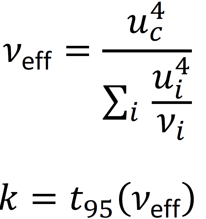
with the coverage factor determined from Student’s t distribution.
For ν = 1 the factor is 12.7 and for ν = 2 it is 4.3; already at ν = 9 it drops to 2.26, and at ν = 30 it has practically reached its asymptotic regime (2.04). In the V-dedicate mode, where the dominant contributions have ν → ∞, k = 2 is directly applicable (Figure B.1).
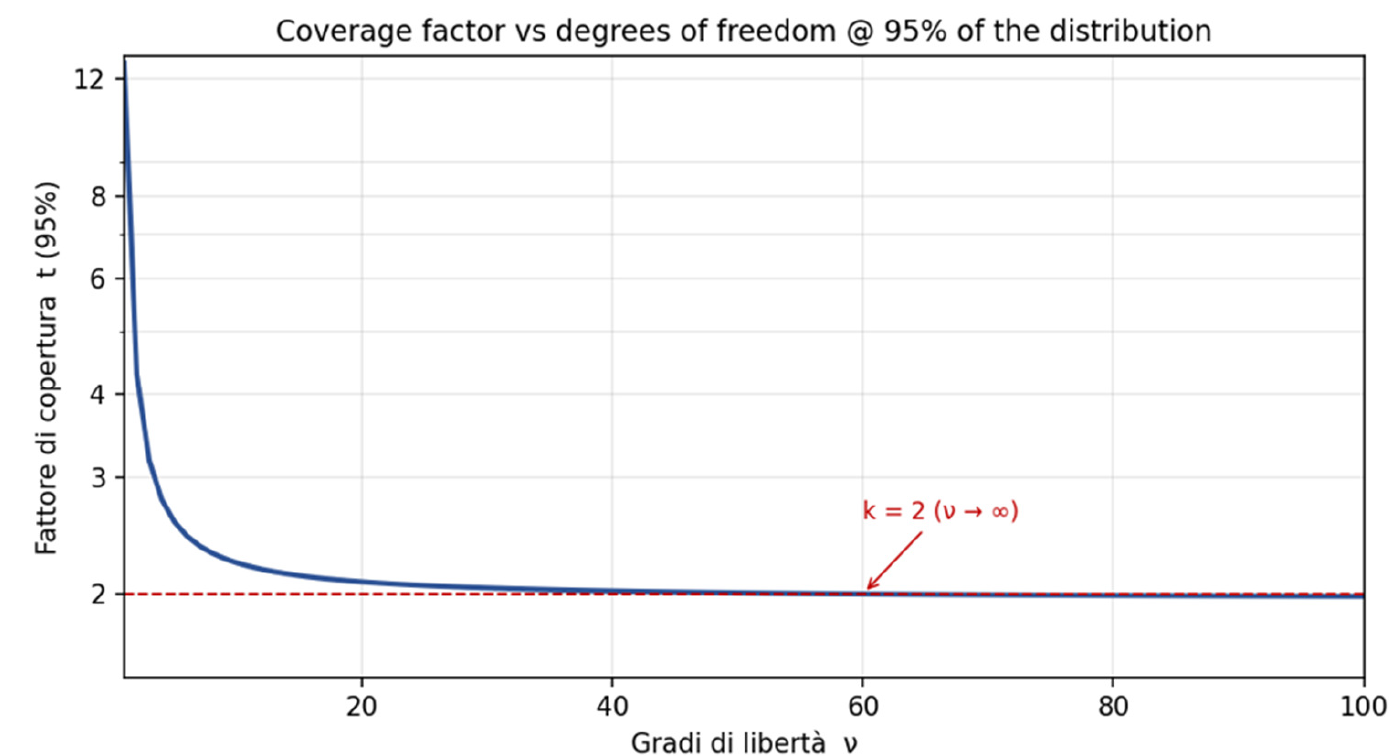
Figure B.1 — Coverage factor at 95% as a function of the degrees of freedom ν (logarithmic vertical scale).
With small samples — in the V-statistic mode e.g. N = 4, ν = 3 — the t factor grows rapidly and the expanded uncertainty may become non-monotonic: as documented in the literature (Ballico 2000; Huang 2018), an intrinsically more precise measurement may turn out to have a larger expanded uncertainty — the so-called «Ballico paradox» (uncertainty paradox), an outcome not justified by the physics of the measurement. This is the known limitation of the WS-t approach for very small samples; for this reason, alongside the WS-t, the JCGM family of documents provides a Bayesian alternative.
Bayesian alternative (JCGM 101:2008 and JCGM 102:2011)
The Bayesian Type A evaluation does not go through the quantile of the t but through the standard deviation of the posterior distribution. Assigning a non-informative prior to the expected value and applying Bayes’ theorem, the posterior distribution of the mean value is a t. In the scalar case (Supplement 1 to the GUM, JCGM 101:2008) the standard uncertainty becomes:
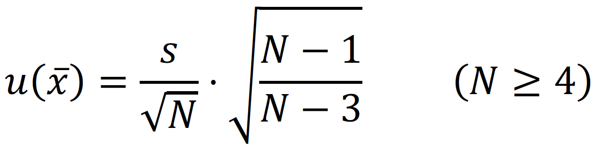
The factor √[(N−1)/(N−3)] is the standard deviation of the t with ν = N−1 degrees of freedom; it is defined only for ν > 2, i.e. N ≥ 4 (at N = 3 the variance of the t diverges). With this factor applied, one combines in quadrature and adopts k = 2.
The same Bayesian setting for Type A is at the core of the draft revision of the GUM (JCGM 100:201X), which makes it the reference method and explicitly addresses the case with fewer than four measurements. A further Bayesian treatment is that of Kacker (“Bayesian alternative to the ISO-GUM's use of the Welch–Satterthwaite formula”).
Table B.1 — Conceptual comparison WS-t vs Bayesian
| Aspect | WS-t | Bayesian |
|---|---|---|
| Normative reference | GUM JCGM 100:2008, Annex G | JCGM 101:2008 (scalar); draft revision JCGM 100:201X |
| Distribution | Student's t with v_eff | t (scalar) t_v(x̄, S/n) |
| Degrees of freedom | v_eff (Welch-Satterthwaite) | v = N - 1 |
Table B.2 — Effective coverage factor at 95% for a Type A contribution
| n | ν | WS-t (k = t95) | Bayesian (k = 2·√[(n−1)/(n−3)]) |
|---|---|---|---|
| 3 | 2 | 4.303 | — (not defined, ν = 2) |
| 4 | 3 | 3.182 | 3.464 |
| 5 | 4 | 2.776 | 2.828 |
| 6 | 5 | 2.571 | 2.582 |
| 10 | 9 | 2.262 | 2.268 |
Both methods are grounded in the t: the WS-t uses it through its quantile, the Bayesian through its standard deviation. Numerically they give very close results (already at n = 6 the difference is ~ 0.4%, while at n = 9 it drops to ~ 0.15%) and converge as n grows. The practical difference emerges with small samples, where the Bayesian is defined only for n ≥ 4 whereas the WS-t remains defined but grows rapidly.
Bibliography
- JCGM 100:2008 — Evaluation of measurement data — Guide to the expression of uncertainty in measurement (GUM).
- JCGM 101:2008 — Supplement 1 to the GUM — Propagation of distributions using a Monte Carlo method (Bayesian Type A evaluation, scalar t distribution).
- JCGM 100:201X — Draft revision of the GUM (committee draft) — Bayesian approach for Type A, including the n < 4 case.
- ISO/IEC 17025:2017 — General requirements for the competence of testing and calibration laboratories (Chapters 6 and 7).
- ILAC G24 — Guidelines for the determination of calibration intervals of measuring instruments.
- ILAC-G8 — Guidelines on decision rules and statements of conformity.
- EURAMET cg-12 — Appendix J (dB / linear / percentage conversions).
- M. Ballico, “Limitations of the Welch–Satterthwaite approximation for measurement uncertainty calculations”, Metrologia 37, 61–64 (2000).
- Huang H. (2016/2018), Uncertainty estimation with a small number of measurements, Measurement Science and Technology / Cal Lab.
- R. N. Kacker, “Bayesian alternative to the ISO-GUM's use of the Welch–Satterthwaite formula”.
Recent

1. IntroductionThe validity of...

The importance of a fully non-magnetic tripod in Shielding Effectiveness (SE) measurements
In Shielding Effectiveness (SE...

ISO 17025 and accredited calibration: what it really means in the context of electromagnetic fields
In the field of electromagneti...

Smoke Detection in MRI Rooms: Fiber Optic Systems for EMI-Free Fire Safety
Smoke detection in magnetic re...

Shielding Effectiveness Measurements: traditional system vs SEMS and calibration criteria
The SEMS (Shielding Effectiven...
Contacts
MPB S.r.l.
Via Giacomo Peroni 400/402
Polo Tecnologico Tiburtino
00131 Roma RM
- Phone:
- +390641200744
- Fax:
- +390641200653
- E-mail:
- info@mpbelectronic.com